Try to find ... similar situation.
You will always find the same solution.
As the heart finds the good thing, the feeling is multiplied.
- Talking Heads "The Good Thing" [Album: More Songs About Buildings and Food]

A goal of this project was to create a searchable code inventory for my personal programming projects. It must be easy to locate programs based on their type and function. With the header and file system information conveniently parsed, validated, and coded to a dictionary of terms, it is time to consider how to efficiently query the data.

Writing and executing SPARQL scripts can be time consuming. If you are creating a solution for a wider audience, it is unlikely they will know SPARQL. There are many approaches to creating a user-friendly interface for graph data. My choice for this exercise is RShiny.

Finding Files with RShiny

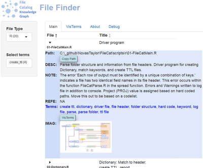
I wrote a custom RShiny interface that allows the user to find files based on file type and term (parsed from the header information). The application is not hosted online. Screen shots of the interface are provided below, along with a link to an example interactive visualization created within the app.

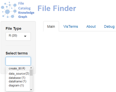
With the data uploaded and the graph database running on localhost, the R code for the app is executed. On the main screen, the user is presented with a drop-down selector to filter the results based on a single file type.

Choices in the selector are populated from a SPARQL query and include the number of files of each FileType, shown in parentheses. ReadMe files and PNG image types are excluded using MINUS because they are not useful in this application.

PREFIX :        <https://www.example.org/tw/filecat#>
PREFIX docdict: <https://www.example.org/tw/filecat/dict#>

SELECT ?fileType (COUNT(?fileType) AS ?count)
WHERE {
   ?file a ?fT .
   MINUS {?file a :FileTypeTXTReadMe}
   MINUS {?file a :FileTypeImagePNG}
   BIND ( REPLACE(STR(?fT), 'https://www.example.org/tw/filecat#|FileType', '') AS ?fileType)    
} GROUP BY ?fileType

The SPARQL file is stored externally from the R Script and read in as an external file. This enables query development and debugging in a separate environment. This is my preferred method for inclusion of SPARQL scripts that do not include parameters selected in the user interface. Here we see the R code snippet that reads-in and executes the query. It then massages the data to include the count of each file type in the drop down selector display.

# Counts of Terms.
queryResult <- SPARQL(url   = ep,
query = read_file('C:/_github/NovasTaylor/FileCat/scripts/sparql/FileTypeCount.rq'))

# Results in FileTypeR, FileTypeRMD, FileTypeSPARQL
fileTypes <- mutate(queryResult$results,
  label = gsub("type", "", paste0(fileType, " (", count,")"), ignore.case = TRUE),
  parameter = paste0("FileType", fileType )) %>%
  select(label, parameter)

A new query is executed immediately after the file type is selected. This query populates the Select Terms box with all terms associated with all files of the selected file type. In the example below, there are four files associated with the bigram “create ttl”, for files that create TTL files as part of their execution. Recall that this catalog is a demonstration of only the files associated with the cataloging project itself, resulting in a smaller number of files and keywords than would be seen in larger code repositories.

The query to produce the list of selected terms relies on the value selected in the File Type selector, so the query statements must exist as a parameterized query within the R code for the Shiny app. The highlighted value in the code below is replaced by the value from the File Type selector:

 terms_query <-  reactive({
  query <- paste0("PREFIX : 
    PREFIX docdict: 
    SELECT ?term (COUNT(?term) AS ?count)
    WHERE {
       ?file a         :FileType", fileType_selected(), " ;
            :filePath  ?path ;
            :hasTerm   ?t .
      BIND ( REPLACE(STR(?t), 'https://www.example.org/tw/filecat/dict#', '') AS ?term)
    } GROUP BY ?term
  ORDER BY ?term")
})

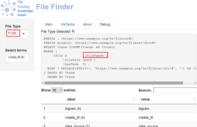
Parameterized queries are more difficult to debug, so a Debug tab was added to the app to display the query with the inserted values and query results. The screen shot below shows how the query contains the selected value for the R File Type :FileTypeR inserted into the query. The query result shows four R files have the associated “create ttl” bigram.

When terms are selected, a table to the right immediately populates with a list of files associated with that term. Selection of multiple terms is possible as an AND condition. For example: create_ttl AND database results in files that only have those two terms.

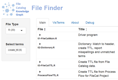
Information about each file is available by clicking on the   icon (not available in the screenshot below.) Users can open the file by copying its full path into an editor and any images documented in the file header are displayed as an expandable thumbnail. This is similar to the Project Catalog, but this table is built using data from the knowledge Graph..

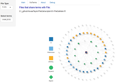
The VisTerms tab provides a visualization of the terms associated with a selected file, files that share terms with the selected file, and terms linked to those files. See the interactive example by clicking the NEXT link at the bottom of this page or the “Example Visualization” link in the chapter table of contents on the left.